Uimhriú sraitheanna uathoibríoch in Excel: 3 bhealach

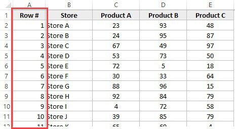
While working in Excel, it is not uncommon to need row numbering in a separate column. This can be done by entering the serial numbers manually, in other words, by typing them on the keyboard. However, when working with a large amount of information, entering numbers manually is not a very pleasant and fast procedure, in which, moreover, errors and typos can be made. Fortunately, Excel allows you to automate this process, and below we will look at exactly how this can be done in various ways.

Modh 1: Uimhriú Tar éis na Chéad Línte a Líonadh

This method is perhaps the easiest. When implementing it, you only need to fill in the first two rows of the column, after which you can stretch the numbering to the remaining rows. However, it is only useful when working with small tables.

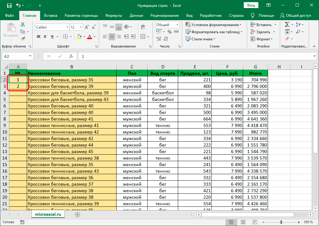
1. First, create a new column for line numbering. In the first cell (not counting the header) we write the number 1, then go to the second, in which we enter the number 2.
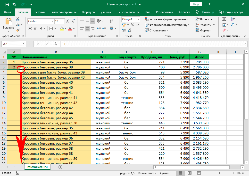
2. Now you need to select these two cells, after which we hover the mouse cursor over the lower right corner of the selected area. As soon as the pointer changes its appearance to a cross, hold down the left mouse button and drag it to the last line of the column.
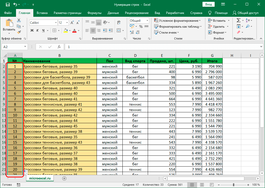
3. We release the left mouse button, and the serial numbers of the lines will immediately appear in the lines that we covered when stretching.

Method 2: STRING operator

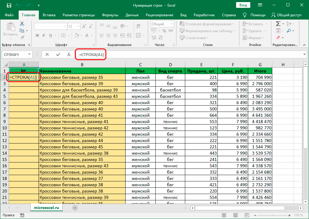
This method for automatic line numbering involves the use of the function “LÍNE”.

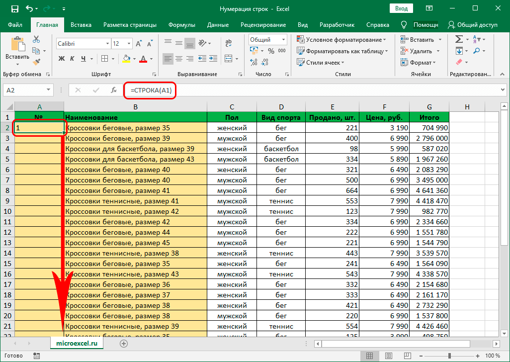
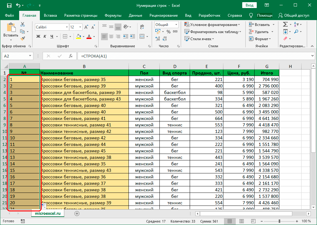
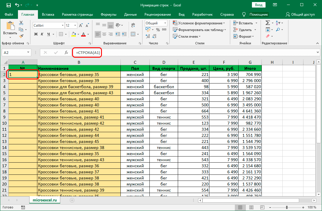
1. We get up in the first cell of the column, which we want to assign the serial number 1. Then we write the following formula in it: =СТРОКА(A1).
2. As soon as we click Iontráil, a serial number will appear in the selected cell. It remains, similarly to the first method, to stretch the formula to the bottom lines. But now you need to move the mouse cursor to the lower right corner of the cell with the formula.
3. Everything is ready, we have automatically numbered all the rows of the table, which was required.

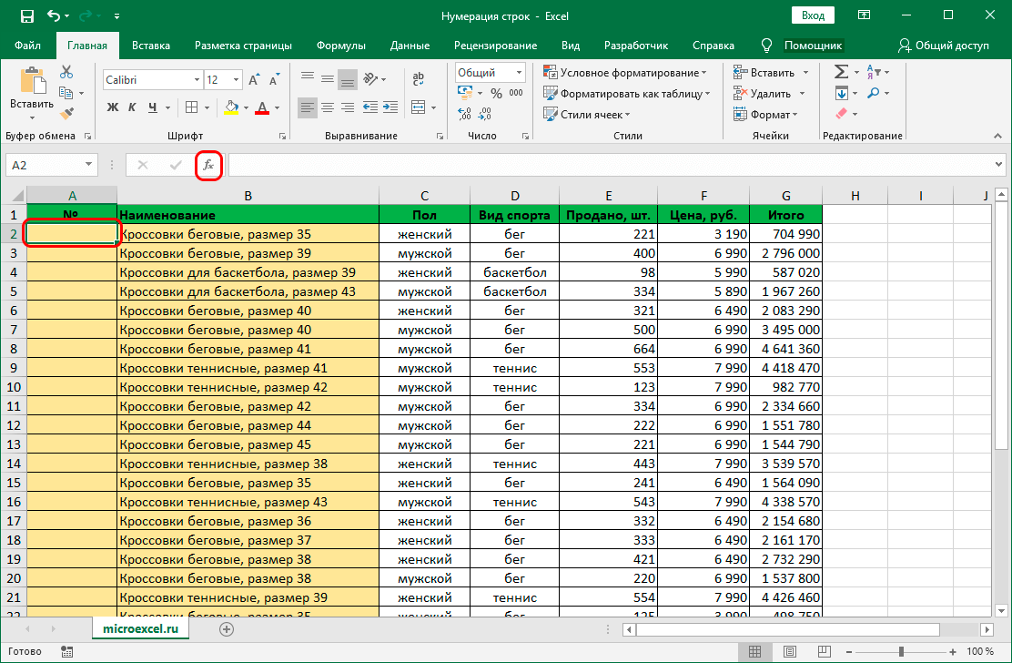
Instead of manually entering the formula, you can use the Function Wizard.

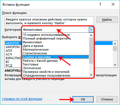
1. We also select the first cell of the column where we want to insert the number. Then we click the button “Cuir isteach feidhm” (ar thaobh na láimhe clé den bharra foirmle).
2. The Function Wizard window opens. Click on the current category of functions and select from the list that opens “References and Arrays”.
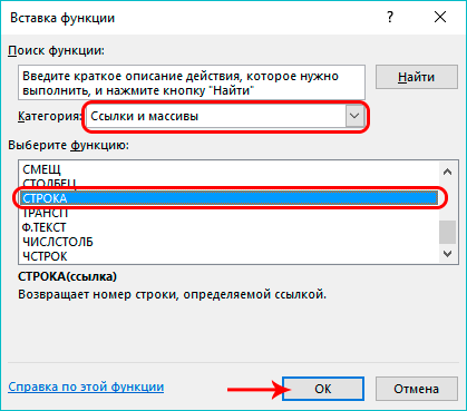
3. Now, from the list of proposed operators, select the function “LÍNE”, ansin brúigh OK.
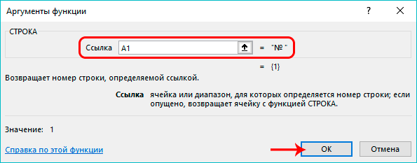
4. A window will appear on the screen with the function arguments to fill in. Click on the input field for the parameter "líne" and specify the address of the first cell in the column to which we want to assign a number. The address can be entered manually or simply click on the desired cell. Next click OK.
5. The row number is inserted in the selected cell. How to stretch the numbering to the rest of the lines, we discussed above.

Modh 3: forchéimniú a chur i bhfeidhm

The downside of the first and second methods is that you have to stretch the numbers to other lines, which is not very convenient for large vertical table sizes. Therefore, let’s look at another way that eliminates the need to perform such an action.

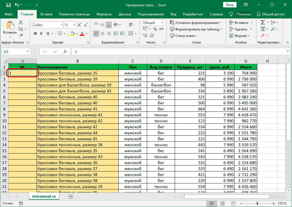
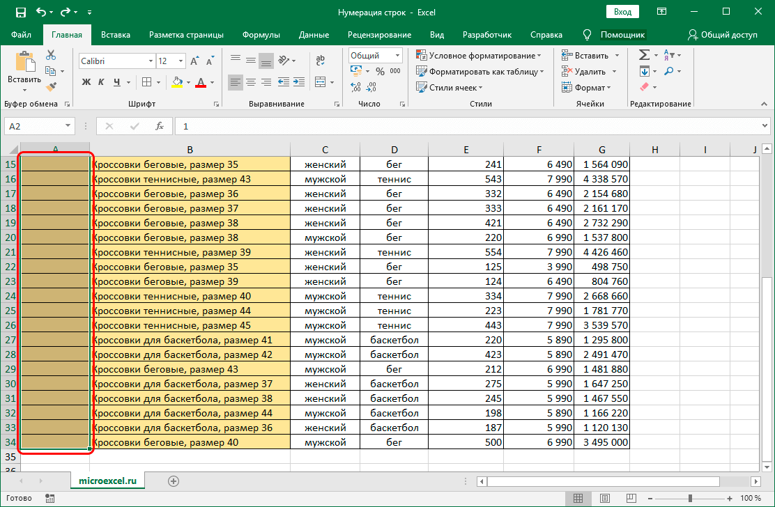
1. We indicate in the first cell of the column its serial number, equal to the number 1.
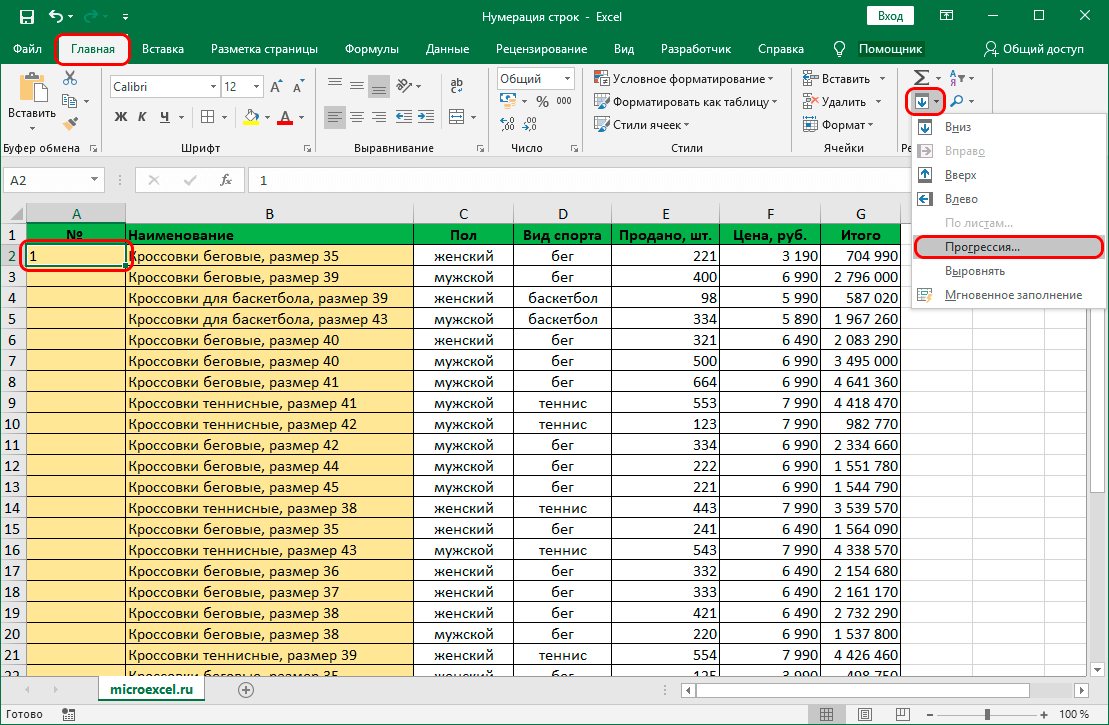
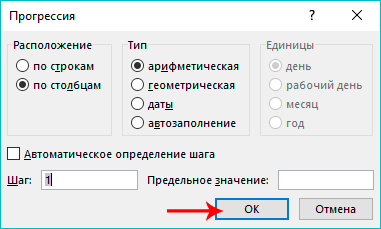
2. Athraigh go cluaisín "Baile", brúigh an cnaipe "Líon" (section “Editing”) and in the list that opens, click on the option “Progression…”.
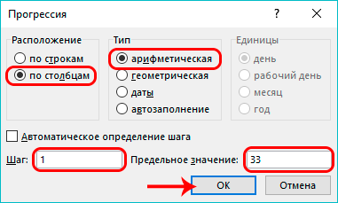
3. A window will appear in front of us with the progression parameters that need to be configured, after which we press OK.
   • select the arrangement “by columns”;
   • specify the type “arithmetic”;
   • in the step value we write the number “1”;
   • in the “Limit value” field, indicate the number of table rows that need to be numbered.
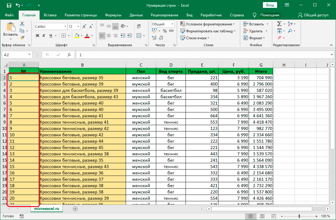
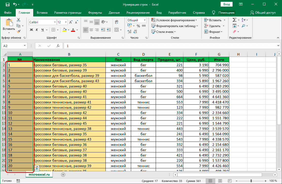
4. Automatic line numbering is done, and we got the desired result.

This method can be implemented in a different way.

1. We repeat the first step, i.e. Write the number 1 in the first cell of the column.
2. We select the range that includes all the cells in which we want to insert numbers.
3. Opening the window again “Progressions”. The parameters are automatically set according to the range we selected, so we just have to click OK.
4. And again, thanks to these simple actions, we get the numbering of lines in the selected range.

The convenience of this method is that you do not need to count and write the number of lines in which you want to insert numbers. And the disadvantage is that, as in the first and second methods, you will have to select a range of cells in advance, which is not so convenient when working with large tables.

Conclúid

Line numbering can make it much easier to work in Excel when working with large amounts of data. It can be done in many ways, ranging from manual filling to a fully automated process that will eliminate any possible errors and typos.